

I remember my first empirical paper like it was yesterday. I had a perfectly valid methodology. I ran a study that made me feel accomplished with a sample that I thought was representative. But I was completely new to statistical methods and empirical research, so, of course, I forgot that I needed to be clear about sample size. And I did not understand the power in my sample. The sinking feeling hit me when R2 asked about my sample size justification and whether I had done a power analysis. A power what now?
Most PhD students spend weeks reading statistical theory, watching YouTube tutorials, and second-guessing themselves about power analysis. They buy expensive statistics software, hire coaches, and still feel uncertain when defending their methodology. Meanwhile, your publication sits untouched while you spiral through Cohen’s 1988 textbook for the third time. The worst part? Your reviewers just want to see you followed standard practices. They’re just checking a box, not testing your statistical prowess.
So, just like I felt an unburdening of worry and the quiet elation that came with it when I knew my statistical efforts were meaningful and correct, I want to show you the exact 5-minute process that gets your power analysis done without the statistical nightmares. And you, too, can feel a sense of pride and relief that the long road of research and writing has led to a successful conclusion with your next publication.
Let’s get this done (fair warning, I’m not a statistician).
Step 1: Download the only free tool you need
First, you need to download the free tool G*Power.
This software has been the gold standard for power analysis since 2007. Universities worldwide accept it. Your reviewers know it. The interface looks dated because it hasn’t changed in years, and that’s actually perfect for us.
Install it on any computer (Windows, Mac, or Linux). The entire program takes up less space than a single PDF textbook. No subscription fees, no hidden costs, no complicated registration process.
Once installed, you’re 4 minutes away from a completed power analysis.
Step 2: Navigate directly to the right calculation
Open G*Power and click these exact options (unless you already know what you’re doing and have done more than a simple comparison of two variables):
- Test family: “t tests”
- Statistical test: “Means: Difference between two independent means (two groups)”
- Type of power analysis: “A priori: Compute required sample size”
These selections work for 90% of beginner studies comparing two groups (but again, if you need to know more, ask you local statistician to explain the details to you). If you’re doing correlational research, select “Correlation: Bivariate normal model” instead. For ANOVA with multiple groups, choose “F tests” then “ANOVA: Fixed effects, omnibus, one-way.”
You can run these statistical tests without learning the underlying mathematical theory. Match your research design to the appropriate test option.
Step 3: Enter these four standard values
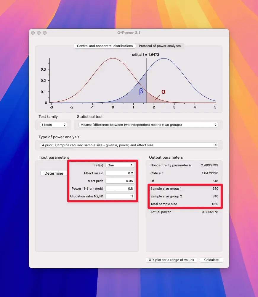
Type these exact numbers:
- Effect size d: 0.2
- α err prob: 0.05
- Power (1-β err prob): 0.80
- Allocation ratio N2/N1: 1
Cohen established 0.5 as a medium effect size in 1988, creating the field’s default standard. But a recent meta-analysis by Gignac and Szodorai (2016) found that Cohen’s benchmarks are arbitrary (small: 0.20, medium: 0.50, large: 0.80) and significantly overestimate typical effect sizes in the psychological literature. The authors recommend using 0.10, 0.20, and 0.30 as new guidelines for small, typical (median), and large effects in psychological research. If you use 0.5 as a typical effect size, you’re overestimating the norm by a wide margin (only a tiny fraction of effects reach that level in their meta-analytic data). For power calculations or interpreting magnitude, the median is closer to 0.2 for Pearson correlations. Fisher introduced the 0.05 alpha level (Type I error probability) in 1925. Statistical power of 0.80 became the standard in the 1970s. Equal allocation between groups maximizes statistical efficiency with a 1:1 ratio.
A word about the standard statistical power threshold of 0.80 though: it means researchers aim for an 80% chance of detecting a real effect if it exists. However, newer research shows that actual effect sizes are typically much smaller than researchers once expected.
For interactions between variables, you should expect regression coefficients (β) or Cohen’s f² values around 0.01 to 0.10. For main effects (meaning: the direct relationship between variables), correlation coefficients (r) typically range from 0.1 to 0.2.
Studies using the traditional 0.80 power threshold miss smaller effect sizes common in psychology research. Most experiments expect effect sizes around d = 0.50, but actual effects often measure d = 0.20 or smaller. When researchers design studies for large effects that don’t exist, their sample sizes become inadequate. A study powered to detect d = 0.50 with 64 participants per group drops to just 33% power when the true effect is d = 0.20. Detecting these realistic smaller effects requires sample sizes of 400+ participants per condition, which now forces researchers to rethink their resource allocation and collaboration strategies.
For GPower power analysis, Lakens (2013) recommends to use Cohen’s dz for within-subjects (paired) comparisons and Cohen’s ds (sometimes labeled simply as d) for between-subjects designs. GPower uses dz as the default effect size for within-subject t-tests. If all of this experiment design lingo sounds scary to you, I recommend starting with the wonderful book: How to Design and Report Experiments by Andy Field and Graham Hole.
The best approach is to use effect sizes from previous research in your research area if available, and only fall back on the classic Cohen guidelines if you genuinely have no better reference. Even then, spell out that you’re using Cohen’s defaults as a last resort, not as strict standards for what counts as practical significance. Just something to keep in mind as the standards here may vary for your field (my field, HCI, is pretty lackadaisical about this standard).
Click “Calculate” and your required sample size appears instantly in the output window. (In the example screenshot above it would be 620 with two samples of 310. And gosh, that’s a lot of people, so you get why most people prefer 0.3 or larger as their effect size, because it cuts that number down more than half or 278 people in total. Put it at 0.5 and you only have to study 102 people.)
Step 4: Add 20% for the real world
Whatever number G*Power gives you, multiply by 1.2.
If G*Power says you need 64 participants (32 per group), your target becomes 77. If it says 128, aim for 154. This buffer accounts for dropouts, incomplete data, and failed manipulation checks. Committee members (and your supervisor) recognize this preparation demonstrates practical research experience.
Round up to the nearest convenient number. Nobody recruits exactly 77 participants. Make it 80. Clean numbers look more professional in your methodology section. But don’t beat yourself up if you don’t meet your goal. At the end the total sample size determines the minimum number you need for your experiment.
Step 5: Write these two methodology sentences
Copy this paragraph exactly (if you’re doing a simple A/B comparison and your results follow a bell curve or normal distribution), and just fill in your numbers:
A priori power analysis using GPower 3.1 indicated a minimum sample size of [GPOWER NUMBER] participants would be needed to detect a median effect size (d = 0.2) with 80% power and an alpha level of .05 for comparing two groups. To account for potential attrition, the target recruitment was increased by 20% to [YOUR INFLATED NUMBER] participants.
That’s your entire power analysis section for a simple beginner study. Done. No complex equations. No theoretical justification. No lengthy explanations.
Handle the only two reviewer questions you’ll get
Reviewers usually ask two predictable questions about power analysis. And it’s usually when you put your effect size somewhere higher between 0.3 and 0.5 (which most researchers do for practical reasons, because most labs cannot afford to run large scale studies). For following, we are assuming an effect size estimate (like 0.3) that’s not conservative but also not outrageous.
Here are your word-for-word responses:
Question 1: Why did you choose your effect size?
Cohen’s 1988 guidelines established 0.5 as a conventional medium effect size, representing a difference that would be practically meaningful in applied settings. A recent meta-analysis by Gignac and Szodorai (2016) confirmed that effect sizes in psychological research typically range from 0.1 to 0.3, making 0.3 a reasonable estimate for our study.
Question 2: What if your actual effect size is smaller?
If the true effect size is smaller than anticipated, this study would be underpowered to detect it. However, effects smaller than d = 0.3 may lack practical significance even if statistically detectable. The chosen effect size balances statistical power with practical relevance, consistent with recommendations by Lakens (2013) for applied research.
Memorize these responses. They end most reviewer discussions quickly.
Skip everything else the textbooks tell you
You don’t need sensitivity analyses. You don’t need power curves. You don’t need to calculate post-hoc power (which statisticians actually hate). You don’t need to justify your alpha level or explain Type I versus Type II error rates. (I mean unless your thesis or paper is actually in statistics, then go hog.)
Your committee has seen hundreds of dissertations. Your reviewers have seen at least dozens of other papers. Must just know the standard approach. Following convention gets you approved faster than trying to impress them with statistical sophistication, but keep in mind the finer points and studies I’ve mentioned here.
The entire process (from downloading G*Power to writing your methodology section) takes 5 minutes. Less time than reading the introduction of a statistics textbook chapter.
Use this approach for these common designs
For correlational studies: Select “Correlation: Bivariate normal model” and use r = 0.30 as your effect size. This gives you 84 participants minimum, or 101 with the buffer.
For three-group comparisons: Choose “ANOVA: Fixed effects, omnibus, one-way” with f = 0.25 effect size and 3 groups. You’ll need 159 participants total, or 191 with buffer.
For regression with 5 predictors: Pick “Linear multiple regression: Fixed model, R² deviation from zero” with f² = 0.15 and 5 predictors. Result: 92 participants, or 111 with buffer.
For repeated measures: Select “Means: Difference between two dependent means (matched pairs)” with d = 0.5. You’ll need 34 participants, or 41 with buffer.
Each calculation takes 30 seconds once you know where to click. And while these may not be the most conservative estimates, they likely get your study rolling.
Start your power analysis right now
Your dissertation methodology chapter needs this completed. Your proposal defence requires it. Your ethics application asks for it.
Open your browser. Download the free tool G*Power. Run your calculation. Write your two sentences. Move on to actually collecting data.
Every day you spend reading about power analysis theory is a day you’re not finishing your dissertation. Or not publishing your papers.
Get it done in 5 minutes. Today.
Bonus Materials
Today, we have a power analysis quick reference template (and Notion cheat sheet), a committee response cheat sheet for your defence, and some sample size calculator shortcuts.